Compressions and Stretches
Learning Outcomes
- Graph Functions Using Compressions and Stretches.
Vertical Stretches and Compressions
When we multiply a function by a positive constant, we get a function whose graph is stretched or compressed vertically in relation to the graph of the original function. If the constant is greater than 1, we get a vertical stretch; if the constant is between 0 and 1, we get a vertical compression. The graph below shows a function multiplied by constant factors 2 and 0.5 and the resulting vertical stretch and compression.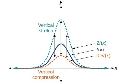 Vertical stretch and compression
A General Note: Vertical Stretches and Compressions
Given a function [latex]f\left(x\right)[/latex], a new function [latex]g\left(x\right)=af\left(x\right)[/latex], where [latex]a[/latex] is a constant, is a vertical stretch or vertical compression of the function [latex]f\left(x\right)[/latex].- If [latex]a>1[/latex], then the graph will be stretched.
- If [latex]0 < a < 1[/latex], then the graph will be compressed.
- If [latex]a<0[/latex], then there will be combination of a vertical stretch or compression with a vertical reflection.
How To: Given a function, graph its vertical stretch.
- Identify the value of [latex]a[/latex].
- Multiply all range values by [latex]a[/latex].
- If [latex]a>1[/latex], the graph is stretched by a factor of [latex]a[/latex]. If [latex]{ 0 }<{ a }<{ 1 }[/latex], the graph is compressed by a factor of [latex]a[/latex]. If [latex]a<0[/latex], the graph is either stretched or compressed and also reflected about the [latex]x[/latex]-axis.
Example: Graphing a Vertical Stretch
A function [latex]P\left(t\right)[/latex] models the number of fruit flies in a population over time, and is graphed below. A scientist is comparing this population to another population, [latex]Q[/latex], whose growth follows the same pattern, but is twice as large. Sketch a graph of this population.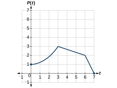
Answer: Because the population is always twice as large, the new population’s output values are always twice the original function’s output values. If we choose four reference points, (0, 1), (3, 3), (6, 2) and (7, 0) we will multiply all of the outputs by 2. The following shows where the new points for the new graph will be located. [latex-display]\begin{cases}\left(0,\text{ }1\right)\to \left(0,\text{ }2\right)\hfill \\ \left(3,\text{ }3\right)\to \left(3,\text{ }6\right)\hfill \\ \left(6,\text{ }2\right)\to \left(6,\text{ }4\right)\hfill \\ \left(7,\text{ }0\right)\to \left(7,\text{ }0\right)\hfill \end{cases}[/latex-display]
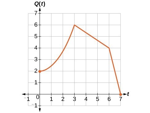 Figure 16
How To: Given a tabular function and assuming that the transformation is a vertical stretch or compression, create a table for a vertical compression.
- Determine the value of [latex]a[/latex].
- Multiply all of the output values by [latex]a[/latex].
Example: Finding a Vertical Compression of a Tabular Function
A function [latex]f[/latex] is given in the table below. Create a table for the function [latex]g\left(x\right)=\frac{1}{2}f\left(x\right)[/latex].| [latex]x[/latex] | 2 | 4 | 6 | 8 |
| [latex]f\left(x\right)[/latex] | 1 | 3 | 7 | 11 |
Answer: The formula [latex]g\left(x\right)=\frac{1}{2}f\left(x\right)[/latex] tells us that the output values of [latex]g[/latex] are half of the output values of [latex]f[/latex] with the same inputs. For example, we know that [latex]f\left(4\right)=3[/latex]. Then [latex-display]g\left(4\right)=\frac{1}{2}\cdot{f}(4) =\frac{1}{2}\cdot\left(3\right)=\frac{3}{2}[/latex-display] We do the same for the other values to produce this table.
| [latex]x[/latex] | [latex]2[/latex] | [latex]4[/latex] | [latex]6[/latex] | [latex]8[/latex] |
| [latex]g\left(x\right)[/latex] | [latex]\frac{1}{2}[/latex] | [latex]\frac{3}{2}[/latex] | [latex]\frac{7}{2}[/latex] | [latex]\frac{11}{2}[/latex] |
Analysis of the Solution
The result is that the function [latex]g\left(x\right)[/latex] has been compressed vertically by [latex]\frac{1}{2}[/latex]. Each output value is divided in half, so the graph is half the original height.Try It
A function [latex]f[/latex] is given below. Create a table for the function [latex]g\left(x\right)=\frac{3}{4}f\left(x\right)[/latex].| [latex]x[/latex] | 2 | 4 | 6 | 8 |
| [latex]f\left(x\right)[/latex] | 12 | 16 | 20 | 0 |
Answer:
| [latex]x[/latex] | 2 | 4 | 6 | 8 |
| [latex]g\left(x\right)[/latex] | 9 | 12 | 15 | 0 |
Horizontal Stretches and Compressions
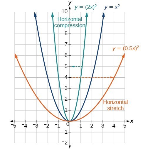 Now we consider changes to the inside of a function. When we multiply a function’s input by a positive constant, we get a function whose graph is stretched or compressed horizontally in relation to the graph of the original function. If the constant is between 0 and 1, we get a horizontal stretch; if the constant is greater than 1, we get a horizontal compression of the function.
Given a function [latex]y=f\left(x\right)[/latex], the form [latex]y=f\left(bx\right)[/latex] results in a horizontal stretch or compression. Consider the function [latex]y={x}^{2}[/latex]. The graph of [latex]y={\left(0.5x\right)}^{2}[/latex] is a horizontal stretch of the graph of the function [latex]y={x}^{2}[/latex] by a factor of 2. The graph of [latex]y={\left(2x\right)}^{2}[/latex] is a horizontal compression of the graph of the function [latex]y={x}^{2}[/latex] by a factor of 2.
Now we consider changes to the inside of a function. When we multiply a function’s input by a positive constant, we get a function whose graph is stretched or compressed horizontally in relation to the graph of the original function. If the constant is between 0 and 1, we get a horizontal stretch; if the constant is greater than 1, we get a horizontal compression of the function.
Given a function [latex]y=f\left(x\right)[/latex], the form [latex]y=f\left(bx\right)[/latex] results in a horizontal stretch or compression. Consider the function [latex]y={x}^{2}[/latex]. The graph of [latex]y={\left(0.5x\right)}^{2}[/latex] is a horizontal stretch of the graph of the function [latex]y={x}^{2}[/latex] by a factor of 2. The graph of [latex]y={\left(2x\right)}^{2}[/latex] is a horizontal compression of the graph of the function [latex]y={x}^{2}[/latex] by a factor of 2.
A General Note: Horizontal Stretches and Compressions
Given a function [latex]f\left(x\right)[/latex], a new function [latex]g\left(x\right)=f\left(bx\right)[/latex], where [latex]b[/latex] is a constant, is a horizontal stretch or horizontal compression of the function [latex]f\left(x\right)[/latex].- If [latex]b>1[/latex], then the graph will be compressed by [latex]\frac{1}{b}[/latex].
- If [latex]0<b<1[/latex], then the graph will be stretched by [latex]\frac{1}{b}[/latex].
- If [latex]b<0[/latex], then there will be combination of a horizontal stretch or compression with a horizontal reflection.
How To: Given a description of a function, sketch a horizontal compression or stretch.
- Write a formula to represent the function.
- Set [latex]g\left(x\right)=f\left(bx\right)[/latex] where [latex]b>1[/latex] for a compression or [latex]0<b<1[/latex] for a stretch.
Example: Graphing a Horizontal Compression
Suppose a scientist is comparing a population of fruit flies to a population that progresses through its lifespan twice as fast as the original population. In other words, this new population, [latex]R[/latex], will progress in 1 hour the same amount as the original population does in 2 hours, and in 2 hours, it will progress as much as the original population does in 4 hours. Sketch a graph of this population.Answer: Symbolically, we could write
[latex]\begin{align}&R\left(1\right)=P\left(2\right), \\ &R\left(2\right)=P\left(4\right),\text{ and in general,} \\ &R\left(t\right)=P\left(2t\right). \end{align}[/latex]
See below for a graphical comparison of the original population and the compressed population.![Two side-by-side graphs. The first graph has function for original population whose domain is [0,7] and range is [0,3]. The maximum value occurs at (3,3). The second graph has the same shape as the first except it is half as wide. It is a graph of transformed population, with a domain of [0, 3.5] and a range of [0,3]. The maximum occurs at (1.5, 3).](https://s3-us-west-2.amazonaws.com/courses-images/wp-content/uploads/sites/896/2016/10/18203623/CNX_Precalc_Figure_01_05_029ab.jpg) (a) Original population graph (b) Compressed population graph
(a) Original population graph (b) Compressed population graphAnalysis of the Solution
Note that the effect on the graph is a horizontal compression where all input values are half of their original distance from the vertical axis.Example: Finding a Horizontal Stretch for a Tabular Function
A function [latex]f\left(x\right)[/latex] is given below. Create a table for the function [latex]g\left(x\right)=f\left(\frac{1}{2}x\right)[/latex].| [latex]x[/latex] | 2 | 4 | 6 | 8 |
| [latex]f\left(x\right)[/latex] | 1 | 3 | 7 | 11 |
Answer: The formula [latex]g\left(x\right)=f\left(\frac{1}{2}x\right)[/latex] tells us that the output values for [latex]g[/latex] are the same as the output values for the function [latex]f[/latex] at an input half the size. Notice that we do not have enough information to determine [latex]g\left(2\right)[/latex] because [latex]g\left(2\right)=f\left(\frac{1}{2}\cdot 2\right)=f\left(1\right)[/latex], and we do not have a value for [latex]f\left(1\right)[/latex] in our table. Our input values to [latex]g[/latex] will need to be twice as large to get inputs for [latex]f[/latex] that we can evaluate. For example, we can determine [latex]g\left(4\right)\text{.}[/latex]
[latex]g\left(4\right)=f\left(\frac{1}{2}\cdot 4\right)=f\left(2\right)=1[/latex]
We do the same for the other values to produce the table below.| [latex]x[/latex] | 4 | 8 | 12 | 16 |
| [latex]g\left(x\right)[/latex] | 1 | 3 | 7 | 11 |
 This figure shows the graphs of both of these sets of points.
Analysis of the Solution
Because each input value has been doubled, the result is that the function [latex]g\left(x\right)[/latex] has been stretched horizontally by a factor of 2.Example: Recognizing a Horizontal Compression on a Graph
Relate the function [latex]g\left(x\right)[/latex] to [latex]f\left(x\right)[/latex].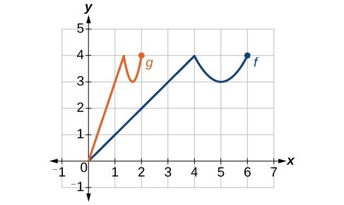
Answer: The graph of [latex]g\left(x\right)[/latex] looks like the graph of [latex]f\left(x\right)[/latex] horizontally compressed. Because [latex]f\left(x\right)[/latex] ends at [latex]\left(6,4\right)[/latex] and [latex]g\left(x\right)[/latex] ends at [latex]\left(2,4\right)[/latex], we can see that the [latex]x\text{-}[/latex] values have been compressed by [latex]\frac{1}{3}[/latex], because [latex]6\left(\frac{1}{3}\right)=2[/latex]. We might also notice that [latex]g\left(2\right)=f\left(6\right)[/latex] and [latex]g\left(1\right)=f\left(3\right)[/latex]. Either way, we can describe this relationship as [latex]g\left(x\right)=f\left(3x\right)[/latex]. This is a horizontal compression by [latex]\frac{1}{3}[/latex].
Analysis of the Solution
Notice that the coefficient needed for a horizontal stretch or compression is the reciprocal of the stretch or compression. So to stretch the graph horizontally by a scale factor of 4, we need a coefficient of [latex]\frac{1}{4}[/latex] in our function: [latex]f\left(\frac{1}{4}x\right)[/latex]. This means that the input values must be four times larger to produce the same result, requiring the input to be larger, causing the horizontal stretching.Try It
Write a formula for the toolkit square root function horizontally stretched by a factor of 3. Use an online graphing calculator to check your work.Answer:
[latex-display]g\left(x\right)=\sqrt{\frac{1}{3}x}[/latex-display]

Licenses & Attributions
CC licensed content, Original
- Revision and Adaptation. Provided by: Lumen Learning License: CC BY: Attribution.
- Question ID 112707, 112726. Authored by: Lumen Learning. License: CC BY: Attribution. License terms: IMathAS Community License CC-BY + GPL.
CC licensed content, Shared previously
- College Algebra. Provided by: OpenStax Authored by: Abramson, Jay et al.. Located at: https://openstax.org/books/college-algebra/pages/1-introduction-to-prerequisites. License: CC BY: Attribution. License terms: Download for free at http://cnx.org/contents/[email protected].
- Question ID 74696. Authored by: Meacham,William. License: CC BY: Attribution. License terms: IMathAS Community License CC-BY + GPL.
- Question ID 60791, 60790. Authored by: Day, Alyson. License: CC BY: Attribution. License terms: IMathAS Community License CC-BY + GPL.
